Retail Sales Forecasting

Note: Current documentation available on the GitHub repository is in Spanish. It will soon be updated to English.
Table of contents
- Introduction
- Objectives
- Understanding the problem
- Project design
- Data quality
- Exploratory data analysis
- Feature engineering and transformations
- Modelling
- Retraining and production scripts
- Conclusion
Introduction
The client is a large American retailer that desires to implement a sales prediction system based on artificial intelligence algorithms.
Notes:
- This article presents a technical explanation of the development process followed in the project.
- Source code can be found here.
Objectives
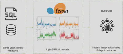
Developing a set of machine learning models on a three-year-history SQL database to predict sales for the next 8 days at the store-product level using massive modelling techniques.
Understanding the problem
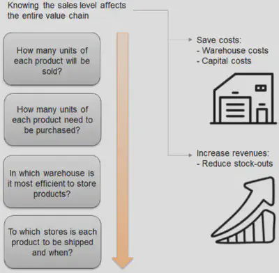
One of the most frequent applications of data science is sales forecasting due to its direct impact on the balance sheet.
Sales forecasting is aimed at improving the following processes:
Supplier relationship management: by having the prediction of customer demand in numbers, it’s possible to calculate how many products to order, making it easy for managers to decide whether the company needs new supply chains or to reduce the number of suppliers.Customer relationship management: customers planning to buy something expect the products they want to be available immediately. Demand forecasting allows to predict which categories of products need to be purchased in the next period from a specific store location. This improves customer satisfaction and commitment to the brand.Order fulfillment and logistics: sales forecasting features optimising supply chains. This means that at the time of order, the product will be more likely to be in stock, and unsold goods won’t occupy prime retail space.Marketing campaigns: forecasting is often used to adjust ads and marketing campaigns and can influence the number of sales. This is one of the use cases of machine learning in marketing. Sophisticated machine learning forecasting models can take marketing data into account as well.Manufacturing flow management: being part of the ERP, the time series-based demand forecasting predicts production needs based on how many goods will eventually be sold.
To this end, traditional sales forecasting methods have been tried and tested for decades. With Artificial Intelligence development, they are now complemented by modern forecasting methods using Machine Learning. Machine learning techniques allows for predicting the amount of products/services to be purchased during a defined future period. In this case, a software system can learn from data for improved analysis. Compared to traditional demand forecasting methods, a machine learning approach allows to:
- Accelerate data processing speed
- Automate forecast updates based on the recent data
- Analyze more data
- Identify hidden patterns in data
- Increase adaptability to changes
Massive and scalable machine learning modelling techniques will be used to approach the present project.
Project design
Project scope, entities and data
This project has been developed based on the data contained in a three-year-history SQL database of a large American retailer. Due to the computational limitations of the equipment available for its development, the scope of the project has been limited to the sales forecasting of ten products belonging to a single category (food) in two different stores. However, the developed system is fully scalable to predict sales of more products, categories and stores by simply changing their respective parameters.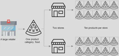
Approach to the main forecasting-related problems
1. Hierarchical Forecasting
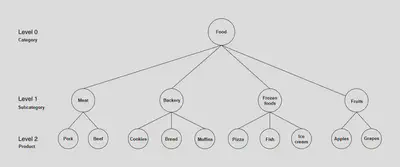
More often than not, time series data follows a hierarchical aggregation structure. For example, in retail, sales for a Stock Keeping Unit (SKU) at a store can roll up to different category and subcategory hierarchies. In these cases, it must be assure that the sales estimates are in agreement when rolled up to a higher level. In these scenarios, Hierarchical Forecasting is used. It is the process of generating coherent forecasts (or reconciling incoherent forecasts) that allows individual time series to be forecasted individually while still preserving the relationships within the hierarchy.
- There are different levels of hierarchies in the commercial catalog.
- It may be interesting to predict sales at different levels.
- Since the forecasts are probabilistic, predictions at different levels will not match exactly.
The forecasts at all of the levels must be coherent. To achieve that, there are different reconciliation approaches to combining and breaking forecasts at different levels. The most common of these methods are as follows:
-
Bottom-Up: in this method, the forecasts are carried out at the bottom-most level of the hierarchy, and then summed going up. For example, in the preceding figure, by using the bottom-up method, the time series’ for the products (level 2) are used to build forecasting models. The outputs of individual models are then summed to generate the forecast for the subcategories. For example, forecasts for ‘apples’ and ‘grapes’ are summed to get the forecasts for ‘fruits’. Finally, forecasts for all of the subcategories are summed to generate the forecasts for ‘food’ category. -
Top-down: in top-down approaches, the forecast is first generated for the top level (‘Food’ in the preceding figure) and then disaggregated down the hierarchy. Disaggregate proportions are used in conjunction with the top level forecast to generate forecasts at the bottom level of the hierarchy. There are multiple methods to generate these disaggregate proportions, such as average historical proportions, proportions of the historical averages, and forecast proportions. -
Middle-out: in this method, forecasts are first generated for all of the series at a ‘middle level’ (for example, ‘meat’, ‘backery’, ‘frozen foods’, and ‘fruits’ in the preceding figure). From these forecasts, the bottom-up approach is used to generate the aggregated forecasts for the levels above this middle level. For the levels below the middle level, a top-down approach is used.
In this case, it has been decided to model at the lowest hierarchical level, i.e. at the store-product level.
2. Intermittent demand
Intermittent demand, also known as sporadic demand, comes about when a product experiences several periods of zero demand. Often in these situations, when demand occurs it is small, and sometimes highly variable in size.
- The source of these zero values is unknown:
- The product was in stock but no sales were made?
- The product was not in stock and therefore could not be sold?
- This situation generates noise and difficulties that worsen the algorithm predictions.
- The optimal way to approach this problem is to get the inventory information in addition to the sales information, thus being able to generate stock-out features that allow the algorithms to discriminate the cause of the zero values.
- If it is not possible to obtain inventory information and/or stock-out marks, another possible approach is to model at a higher hierarchical level, especially if the products are in very low demand.
- It is also possible to create synthetic features that try to identify whether or not stock-outs have occurred.
- Employing forecasting methods based on machine learning techniques, which are less sensitive to these problems than classical approaches.
- Employing more advanced methodologies such as:
- Croston method and derivatives.
- ML models to predict the probability that a particular day’s sales will be zero.
In the present project, there is no inventory information or stock-out marks available in the provided database, so it has been decided to generate synthetic features that collect the situations where stock-outs occur based on business rules.
3. There are hundreds or thousands of Stock Keeping Units (SKUs)
In real contexts and sectors such as retail, ecommerce, there are often thousands of different products for which to predict the sales level.
- Depending on the number of SKUs, the desired level of temporal aggregation (hourly/daily/weekly models…), the amount of historical data being used, the computational resources available, etc., there may come a point where modelling process is not computationally feasible.
- Employing the forecasting approach based on machine learning, since once the models are trained, it is much faster than the classical approach.
- Using faster models such as LightGBM.
- Modelling at a higher hierarchical level and estimate the forecast of the lower levels by applying top-down reconciliation techniques.
- Using big data techniques to train the models
- Powerful cloud machines.
- Big Data clusters.
Forecasting approach based on machine learning and LightGBM tree-based algorithm architecture has been employed in the project.
Data quality
In this stage of the project, general data quality correction processes have been applied, such as:
- Feature renaming
- Feature type correction
- Elimination of features with unique values
- Nulls imputation
- Outliers management
- …
The entire process can be consulted in detail here.
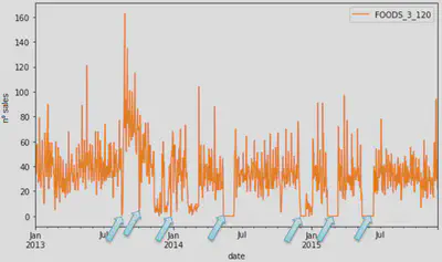
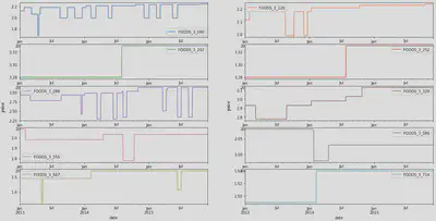
Exploratory data analysis
The aim of this stage of the project is to discover trends, patterns, and to check assumptions with the help of statistical summary and graphical representations. Complete analysis can be found here.
Example of the analysis of some of the analysis that have been conducted:
Feature engineering and transformations
At this stage of the project, different variable transformation techniques (one hot encoding, target encoding, etc.) have been applied to adapt them to the requirements of the algorithms that will be used during the modelling phase.
On the other hand, aiming to increase the predictive capacity of the models, new features have been created, such as:
Intermittent demand features: explained at project design section.Lag features: are values at prior timesteps that are considered useful because they are created on the assumption that what happened in the past can influence or contain a sort of intrinsic information about the future.Rolling window features: the main goal of building and using rolling window features in a time series dataset is to compute statistics on the values from a given data sample by defining a range that includes the sample itself as well as some specified number of samples before and after the sample used.
Complete source code of this stage can be found here.
Modelling
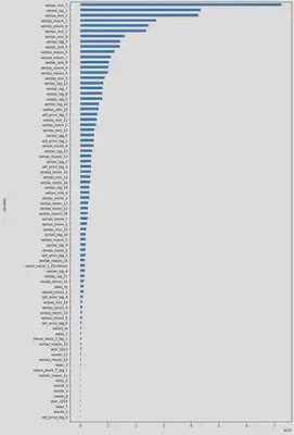
Feature selection
At this stage of the project most predictive features have been analysed by comparing the results of three different selection methods (Recursive feature elimination, Mutual information, Permutation importance), to both improve the performance of the models and reduce the computational modelling costs. Finally, the 70 most predictive features identified by ‘Recursive feature elimination’ method have been selected. Entire feature selection code is available here.
Developing a one-step forecasting model for a specific product-store combination
The objective of this stage of the project is not to obtain the final models but to design the modeling process (algorithm selection, hyperparameter optimization, model evaluation...) for the minimum analysis unit (product-store), in order to verify the correct functioning of the process and to avoid possible error sources when scaling the one-step forecasting process to all product-store combinations.In order to prevent overfitting and evaluate model performance in a more robust way than simple train-test, a cross validation strategy has been implemented.
In the case of time series, the cross-validation is not trivial. Random samples can not be assigned to either the test set or the train set because it makes no sense to use the values from the future to forecast values in the past. In simple word future-looking must be avoided when training the models. There is a temporal dependency between observations that must be preserved during testing.
The method that can be used for cross-validating the time-series model is cross-validation on a rolling basis. Start with a small subset of data for training purpose, forecast for the later data points and then checking the accuracy for the forecasted data points. The same forecasted data points are then included as part of the next training dataset and subsequent data points are forecasted.
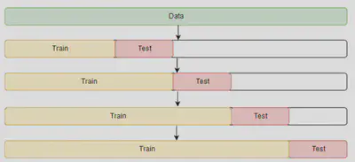
In the present project the cross validation process has been implemented using sklearn.model_selection.TimeSeriesSplit class of scikit-learn package with 3 splits and 8 days as maximum training size.
As discussed in the general design phase of the project, the algorithmic architecture used to implement the different models has been LightGBM given its favorable relationship between predictive capability and the computational time required.
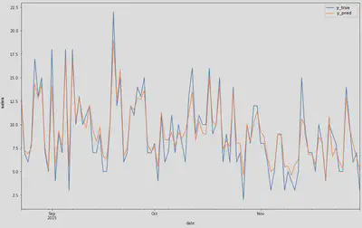
Different combinations of hyperparameters have been tested to find those with the best performance. Evaluation scores obtained in the tested parametrisations remains stable during cross-validation process, which is a good indicator of the stability of the model predictions.
The objective here is not to evaluate the model quality (since the predictions have been made using the training data), but simply to verify that the process works properly, that the order of magnitude of the predictions is correct and that no other anomalous behavior are detected before moving on with the project.
Generalizing the one-step forecasting model creation process
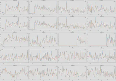
Once the model generation process has been created and polished at the individual level (product-store), in this section the code necessary to scale this process to all the products to be modeled has been developed.
Again, the objective here is not to evaluate quality of the models but simply to verify that the generalization of the one-step forecasting model creation process works properly.
Recursive multi-Step Time Series Forecasting
At this point of the project it has been designed a scalable process of one-step forecasting model generation, thus being able to predict the next day’s sales at product-store level. However, the project’s objective is to make these predictions not only for the next day but for the following 8 days.
Predicting multiple time steps into the future is called multi-step time series forecasting. There are several approaches to this problem, of which the two main ones are as follows:
-
Direct Multi-step Forecast Strategy: The direct method involves developing a separate model for each forecast time step. Having one model for each time step is an added computational and maintenance burden. On the other hand, because separate models are used, it means that there is no opportunity to model the dependencies between the predictions, such as the prediction on day 2 being dependent on the prediction in day 1, as is often the case in time series.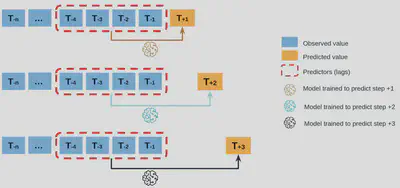
Direct Multi-step Forecast strategy. -
Recursive Multi-step Forecast: The recursive strategy involves using a one-step model multiple times where the prediction for the prior time step is used as an input for making a prediction on the following time step, being therefore a better approximation than the direct one with respect to computational and maintenance aspects. However, the recursive strategy allows prediction errors to accumulate such that performance may quickly degrade as the prediction time horizon increases.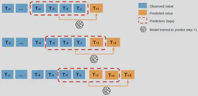
Recursive Multi-step Forecast strategy.
Recursive multi-step forecasting approach has been finally implemented in order to reduce as much as possible the development and maintenance costs of the models.
Complete modelling process can be consulted here.
Retraining and production scripts
Once all recursive multi-step forecasting models have been developed, trained and evaluated properly, in this final stage of the project all the necessary processes, functions and code have been compiled in a clean and optimal way into two Python scripts:
- Retraining script: automatically retrains all developed models with new data when necessary.
- Production script: executes all models and obtains the results.
Conclusion
Warehouse costs and stock-outs have been reduced by developing a scalable set of machine learning models that predict the demand in the next 8 days at store-product level.
Pedro Cortés Macías
Data scientist · Industrial Engineer
I love solving problems. More specifically, I love solving problems using code, maths and business knowledge. Using it for analysis and automation, helping people and companies to be more productive, make better decisions and create data-driven assets.