Credit Risk Scoring

Introduction

---

The client is an online platform which specialises in lending various types of loans to urban customers. Borrowers can easily access lower interest rate loans through a fast online interface.

When the company receives a loan application, the company has to make a decision for loan approval based on the applicant’s profile. Like most other lending companies, lending loans to ‘risky’ applicants is the largest source of financial loss. The company aims to identify such ‘risky’ applicants and their associated loan’s expected loss in order to utilise this knowledge for managing its economic capital, portfolio and risk assessment.

Notes:

• This article presents an overview of the development process followed in the project.
• Source code can be found here.
• Feel free to test the developed credit risk analyzer web application here.

Objectives

---

Creating an advanced analytical asset based on machine learning predictive models to estimate the expected financial loss of each new customer-loan binomial.

Understanding the problem

---

Credit risk is associated with the possibility of a client failing to meet contractual obligations, such as mortgages, credit card debts, and other types of loans.

Minimizing the risk of default is a major concern for financial institutions. For this reason, commercial and investment banks, venture capital funds, asset management companies and insurance firms are increasingly relying on technology to predict which clients are more prone to stop honoring their debts. Accounting for credit risk in the entire portfolio of instruments must consider the likelihood of future impairment and is commonly measured through expected loss and lifetime expected credit loss. To comply with IFRS 9 or CECL, risk managers need to calculate the expected credit loss on the portfolio of financial instruments over the lifetime of the portfolio.

Machine Learning models have been helping these companies to improve the accuracy of their credit risk analysis, providing a scientific method to identify potential debtors in advance.

Project design

---

Methodology

In order to estimate the expected loss (EL) associated to a certain loan application, three essential risk parameters have been considered:

• Probability of default (PD): is a measure of credit rating that is assigned internally to each customer with the aim of estimating the probability that a given customer will default.
• Loss given default (LGD): is another of the key metrics used in quantitative risk analysis. It is defined as the percentage risk of exposure that is not expected to be recovered in the event of default.
• Exposure at default (EAD): is defined as the percentage of outstanding debt at the time of default.

Three predictive machine learning models will be developed to estimate these risk parameters, and their predictions will be combined to estimate the expected loss of each loan transaction as follows:

$$ EL\,(\$) = PD (\%) \cdot P (\$) \cdot EAD (\%) \cdot LGD (\%) $$ where P is the loan principal (the amount of money the borrower wishes to apply for).

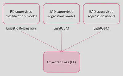
Note that the model for estimating the probability of default will be developed using a logistic regression algorithm. ‘Black box algorithms’ are not suitable in regulated financial services as their lack of interpretability and auditability could become a macro-level risk and in some cases, the law itself may dictate a degree of explainability. To overcome this problem, a highly explainable AI model, such as logistic regression, which provide details or reasons to make the functioning of AI clear or easy to understand, will be applied.

For the case of the exposure at default and loss given default models, different combinations of algorithms (Ridge, Lasso, LightGBM…) and hyperparameters have been tested to find those with the best performance. LightGBM algorithm was finally choosen in both cases.

Entities and data

The data under analysis is available at Lending Club website and contains information collected by the company regarding two main entities:

1. Borrowers: There are features in the dataset capturing information on the applicant profile, i.e. applicant employment history, number of mortgages and credit lines, annual incomes and other personal information.

2. Loans: The rest of the features provide information on the loan such as loan amount, loan interest rate, loan status (i.e. whether the loan is current or in default), loan tenor (either 36 or 60 months) between others.

Data quality

---

In this stage of the project, general data quality correction processes have been applied, such as:

• Feature renaming
• Feature type correction
• Elimination of features with unique values
• Nulls imputation
• Outliers management

The entire process can be consulted in detail here.

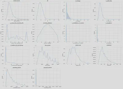
Exploratory data analysis

---

The aim of this stage of the project is to discover trends, patterns, and to check assumptions with the help of statistical summary and graphical representations. Complete analysis can be found here.

In order to guide the process, a series of seed questions were posed to serve as a basis for developing and deepening the analysis of the different features.

Seed questions

Regarding Borrowers:

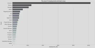
• Q1: What are the most frequent professions of clients applying for loans?

• Q2: How is the score feature assigned by the company to each applicant performing?

• Q3: Can different customer behaviour profiles be distinguished with regard to the way they use their credit cards?

Regarding Loans:

• Q4: Regarding the percentage of late payments and carged-offs, are there differences between 36 and 60 month loans?

• Q5: Can specific loan purposes be identified as more likely to default than others?

Some of the analyses carried out in this data exploration phase are shown below.

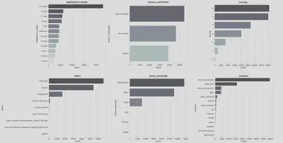
Insights

Borrowers:

• Borrowers with poorer credit scores tend to borrow larger amounts and have lower annual incomes than clients with higher credit scores, thus paying higher monthly installments and higher interest rates.
• One third of all customers have been employed for more than 10 years. The job title of most clients is unknown. Of the clients who do provide this information, the top three most frequent jobs are ‘Teacher’, ‘Manager’ and ‘Owner’.
• The score feature appears to be predictive of loan status: the percentage of loans charged off increases as the borrower’s credit score worsens while the percentage of fully paid loans increases as the borrower’s credit score increases.
• Three main groups can be clearly distinguished: those borrowers who used less than 20% of the credit available on their credit card, another group of borrowers have used between 20 and 80 percent of the available credit on their credit card, and a last group of borrower who have used more than 80% of their available credit on their credit card.

Loans:

• In general, 60-month loans tend to have a higher percentage of late payments and charge-offs.
• The percentage of loans charged off for ‘moving’ and ‘small business’ purposes is slightly higher (16%-17%) than the average for the rest of loan purposes (around 11%).

Feature transformation

---

At this stage of the project, different feature transformation techniques will be applied to adapt them to the requirements of the algorithms that will be used during the modelling phase. Detailed process can be found here.

As discussed prevously, three different models will be developed:

• PD: Probability of default model.
• EAD: Exposure at default model.
• LGD: Loss given default model.

In all cases, categorical features have to be transformed into numerical features. Ordinal encoding, one hot encoding and target encoding techniques will be employed for this purpose. Note that as target encoding process is target-dependent, 3 different transformations must be carried out, one for each of the models to be developed.

Regarding continuous features, given that PD model will be implemented using a logistic regression algorithm (as discussed in previous stages of the project), Gaussian normalisation processes will be applied.

Finally, feature rescaling processes will be applied to transform all features in the dataset to a shared 0-1 scale.

Defining and creating targets

The second major objective of this section is the definition and creation of the target for each of the models to be developed.

Probability of default (PD):

The purpose of this model will be to predict the probability that a given customer will default. In the context of this project, a default will be defined as any delay in the payment of loan installments of more than 90 days.

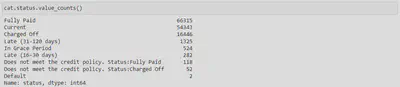
During the exploratory data analysis phase, it was found that ‘Charged off’ and ‘Does not meet the credit policy. Status:Charged Off’ loan status categories had to be considered as default as certain amounts had been recovered in them. Obviously, ‘Default’ category should also be considered as default. By other hand, ‘Current’, ‘Fully Paid’, ‘In Grace Period’ and ‘Does not meet the credit policy. Status:Fully Paid’ categoires will clearly not be considered as non-payments.

Regarding ‘Late (31-120 days)’ category and due to the selected criterion of considering >90 days = default, a decision should be made whether to include this category as default or not. Given that no additional information is available, it has been decided not to consider this category as default as 66% of its range is below 90 days

Taking into account all of the above, a binary target is created, where class 1 indicates the cases considered as default.

Loss given default (LGD):

The objective of this model is to predict the percentage of the loan that a given borrower has not yet repaid when a default occurs. The target for this model can thus be defined as:

$$ \text{target}_{\text{ead}} = \dfrac{\text{Amount to be paid}}{\text{Loan amount}} = \dfrac{\text{Loan amount} - \text{Amortised amount}}{\text{Loan amount}} $$

Exposure at default (EAD):

The objective of this model is to predict the percentage of the principal that will not be possible to recover from a loan that has been defaulted on. Therefore, the target for this model will be defined as:

$$ \text{target}_{\text{lgd}} = \begin{cases} \dfrac{\text{Recovered amount}}{\text{Amount to be paid}} & if \, \text{Amount to be paid} > 1 \\ 0 & if \, \text{Amount to be paid} = 0 \end{cases} $$

Modelling

---

Probability of default model (PD)

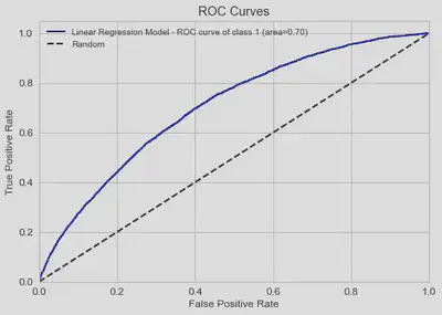
As discussed in the design stage of the project, probability of default (PD) model will be based on the logistic regression algorithm. This stage aims to find the optimal combination of hyperparameters for this algorithm arquitecture.

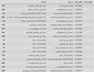
As already detected during the exploratory analysis phase, there is a high correlation between scoring and interest_rate features, as well as between loan amount and the monthly installments. After an iterative modelling process, it is found that the scoring and loan_amount features are more predictive than interest_rate and installment, so only the first two will be used in order to avoid these high correlations.

The remaining correlations are mainly due to the one hot encoding process. Lasso-regularised algorithm settings will preferably be selected to mitigate these effects.

Once the hyperparameter optimisation process has been carried out, in which different penalty strengths and strategies have been tested (l1, l2, elasticnet, none), it is found that the best parameterisation corresponds to a logistic regression with lasso regularisation, which obtains an ROC-AUC value of 0.7 on the test data.

On the other hand, through the coefficient analysis of the trained logistic regression model, it is observed that the features that most strongly determine the customer’s probability of default are the customer’s credit score, employment, number of credit lines and annual income.

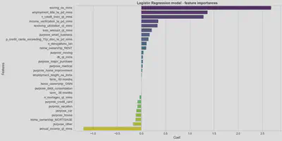
Note: complete development process of the PD model can be consulted here.

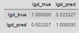
Loss given default model (LGD)

At this stage different combinations of algorithms (Ridge, Lasso, LightGBM) and hyperparameters have been tested to find those with the best performance. It is found that LightGBM architecture is the one that is performing best.

As can be seen, the error made by the model in predicting the level of not amortised loan when default occurs is high. Nevertheless, it should be noted that errors in this type of risk acquisition models are generally significantly higher than those in behavioural models, marketing, customer management, etc., as much less customer information is available when running the model.

In the same vein, it should also be noted that both defaulting and non-defaulting borrowers are being modelled, as this information is not available for a new customer. Therefore, on many occasions the model will be trying to predict the exposure at default of borrowers who are unlikely to default, which also explains the level of errors obtained in the modelling.

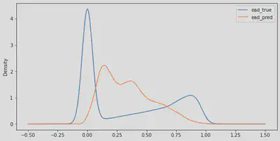
It can be seen that in reality (ead_true) three large groups can be distinguished, a majority group of borrowers whose exposure to default is zero, a second group with intermediate exposures (0.25-0.75), and a last group where all those borrowers with greater exposure to default are concentrated.

Model’s predictions tend towards intermediate default exposures, which leads to larger errors in predicting those borrowers with very low or very high actual default exposures.

• For customers who will actually have very limited exposures at default: the model predicts that they will have some degree at exposure to default, which will lead to somewhat higher fees/interest being charged than they would be entitled to.
• For customers with high actual default exposures: the model will tend to predict lower than actual default exposures, so that lower fees/interest will be applied than would be the case.

However, at an aggregate level from a business point of view the performance of the model is quite acceptable, as it will be covering the part of fees/interest not collected from borrowers who end up having high exposure defaults with the additional surcharges/interest charged to those customers who eventually did not have defaults, thus covering the aggregate risk of the client portfolio.

Note: complete development process of the LGD model can be consulted here.

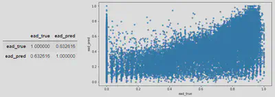
Exposure at default model (EAD)

Similar to the process carried out in the LGD model, different parametrisations of Ridge, Lasso and LightGBM algorithms have been tested, and again LightGBM architecture provides the best results.

The error of this model is relatively high, which is explained for the same reasons exposed previously (as it is also a risk acquisition model with limited features available to make predictions).

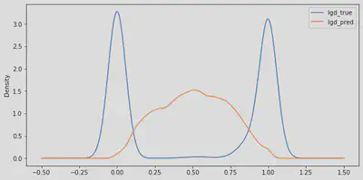
It can be seen that in reality (lgd_true) two large groups can be distinguished: a group of loans in which no amount is recovered, either because the borrower has not defaulted or because the borrower has defaulted but the bank has not been able to recover any amount; and a second group of loans in which it has been possible to recover the full amount, either because the borrower has amortised the entire loan or because it has been possible to recover the full amount a defaulted loan.

Model’s predictions tend towards intermediate loss levels, which leads to larger errors in predicting fully recovered or lost loans.

However, as presented for LGD model, the performance of the EAD model is acceptable at an aggregate level from a business point of view, as it will be covering the lost amount of loans in which the amount borrowed has been completely lost by predicting to most customers a loss level of between 25% and 75% even those who ultimately fully paid their loans, thus covering the aggregate risk of the client portfolio.

Note: complete development process of the EAD model can be consulted here.

Final Expected Loss model (EL)

Once the probability of default, exposure at default and loss given default models have been developed, the expected loss (EL) for each new loan application is obtained by simply combining the predictions of these models and the principal amount of the loan as discussed in the methodology section.

$$ EL\,(\$) = PD (\%) \cdot P (\$) \cdot EAD (\%) \cdot LGD (\%) $$

Model deployment - Web app

---

In order to get the most value out of the developed machine learning models, it is important to seamlessly deploy it into production so employees can start using them to make practical decisions.

To this end, a prototype web application has been designed. This web app collects, on the one hand, the internal data that the company has for each client and on the other hand, the information provided by the borrower itself through a loan application.

• Launch Credit Risk Analyzer Web App!

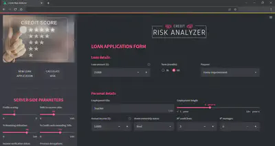
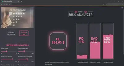
Once the data has been entered, by clicking on “CALCULATE RISK” button, the application will run the machine learning models on the data and will return the expected loss of the loan application as well as the probability of default, loss given default and exposure at default KPIs.